Also see GitHub Reop on Statistical tests in Data Science

Statistical Tests: When to Use Them, Assumptions, and SciPy Links

Quick Decision Rule

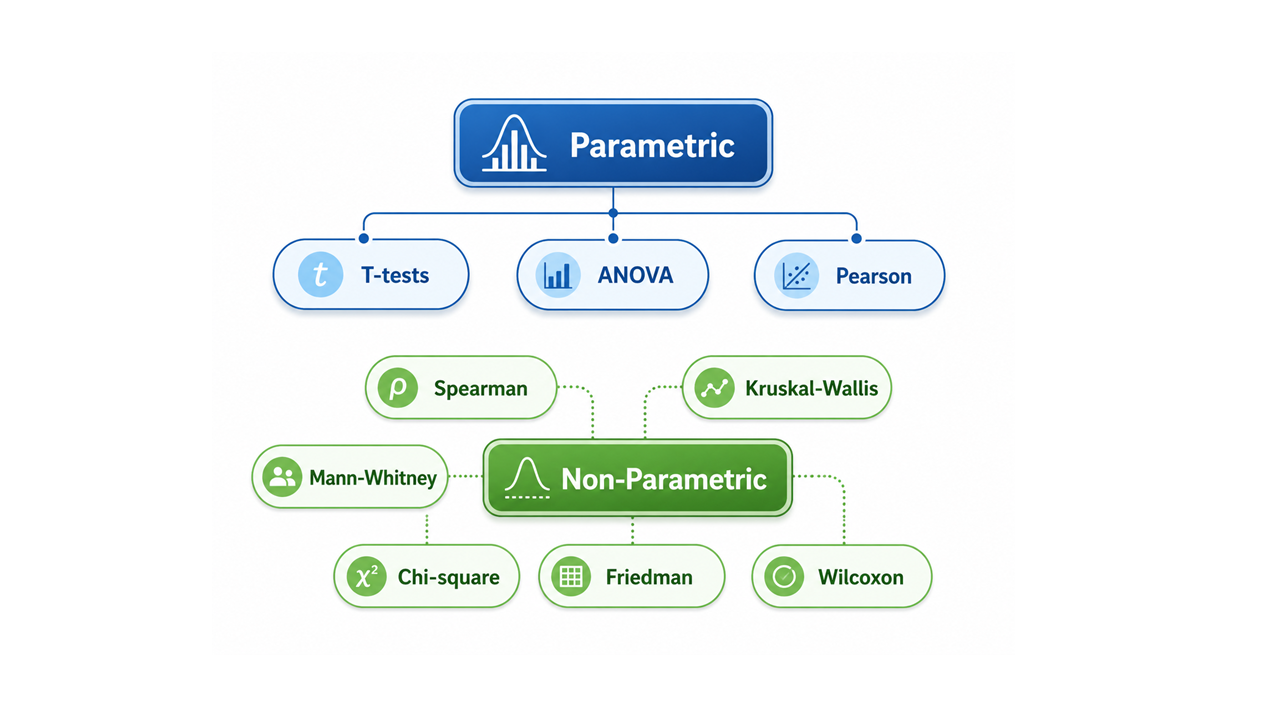
Situation	Test
2 independent groups + numeric outcome + normal data	Independent t-test
3+ independent groups + numeric outcome + normal data	One-way ANOVA
2 independent groups + numeric outcome + non-normal data	Mann-Whitney U test
3+ independent groups + numeric outcome + non-normal data	Kruskal-Wallis test
2 paired/repeated measurements + non-normal data	Wilcoxon signed-rank test
3+ paired/repeated measurements + non-normal data	Friedman test
Category vs category	Chi-square test of independence
Two numeric variables + linear relationship + normal-ish data	Pearson correlation
Two numeric/ordinal variables + monotonic or non-normal relationship	Spearman correlation
Check whether numeric data is normally distributed	Shapiro-Wilk test

---

1. Independent Samples t-test

SciPy function: scipy.stats.ttest_ind
Official documentation: https://docs.scipy.org/doc/scipy/reference/generated/scipy.stats.ttest_ind.html

When to use

Use an independent samples t-test when you want to compare the mean of a numeric variable between two independent groups.

Example question

Do male and female students differ in their mean exam scores?

Variables

• Group variable: gender → Male / Female
• Outcome variable: exam_score → numeric

Hypotheses

• H0: The two group means are equal.
• H1: The two group means are different.

Assumptions

1. The dependent variable is numeric.
2. The two groups are independent.
3. The dependent variable is approximately normally distributed within each group.
4. The variances of the two groups are equal if using the classic Student t-test.
5. If variances are not equal, use Welch’s t-test by setting equal_var=False.

Related assumption checks

• Normality: scipy.stats.shapiro
• Equal variance: scipy.stats.levene

Example code

from scipy.stats import ttest_ind, shapiro, levene

male = df.loc[df["gender"] == "Male", "exam_score"]
female = df.loc[df["gender"] == "Female", "exam_score"]

# normality
print(shapiro(male))
print(shapiro(female))

# equal variance
lev_stat, lev_p = levene(male, female, center="median")

# t-test
t_stat, p_value = ttest_ind(
    male,
    female,
    equal_var=lev_p > 0.05,
    nan_policy="omit",
    alternative="two-sided"
)

print(t_stat, p_value)
````

---

## 2. One-way ANOVA

**SciPy function:** `scipy.stats.f_oneway`
**Official documentation:** [https://docs.scipy.org/doc/scipy/reference/generated/scipy.stats.f_oneway.html](https://docs.scipy.org/doc/scipy/reference/generated/scipy.stats.f_oneway.html)

### When to use

Use one-way ANOVA when you want to compare the **mean** of a numeric variable across **three or more independent groups**.

### Example question

Do Online, Classroom, and Hybrid teaching methods differ in mean exam scores?

### Variables

* Group variable: `teaching_method` → Online / Classroom / Hybrid
* Outcome variable: `exam_score` → numeric

### Hypotheses

* H0: All group means are equal.
* H1: At least one group mean is different.

### Assumptions

1. The dependent variable is numeric.
2. Groups are independent.
3. The dependent variable is approximately normally distributed within each group.
4. The group variances are approximately equal, also called homoscedasticity.

### Related assumption checks

* Normality: `scipy.stats.shapiro`
* Equal variance: `scipy.stats.levene`

### Example code

from scipy.stats import f_oneway, shapiro, levene

groups = [ group["exam_score"].dropna() for name, group in df.groupby("teaching_method") ]

normality for each group

for name, group in df.groupby("teaching_method"): print(name, shapiro(group["exam_score"].dropna()))

equal variance

print(levene(*groups, center="median"))

ANOVA

f_stat, p_value = f_oneway(*groups)

print(f_stat, p_value)

### Important note

ANOVA tells you whether **at least one group differs**, but it does not tell you exactly **which groups differ**. If ANOVA is significant, use a post-hoc test such as Tukey HSD.

---

## 3. Mann-Whitney U Test

**SciPy function:** `scipy.stats.mannwhitneyu`
**Official documentation:** [https://docs.scipy.org/doc/scipy/reference/generated/scipy.stats.mannwhitneyu.html](https://docs.scipy.org/doc/scipy/reference/generated/scipy.stats.mannwhitneyu.html)

### When to use

Use Mann-Whitney U when you want to compare **two independent groups**, but the numeric outcome is **not normally distributed** or is ordinal.

### Example question

Do male and female students differ in screen time?

### Variables

* Group variable: `gender` → Male / Female
* Outcome variable: `screen_time` → numeric but skewed

### Hypotheses

* H0: The two groups come from the same distribution.
* H1: The two groups come from different distributions.

### Assumptions

1. The dependent variable is numeric or ordinal.
2. The two groups are independent.
3. Observations are independent.
4. The distributions should have a similar shape if you want to interpret the result as a median/location difference.

### Example code

from scipy.stats import mannwhitneyu

male = df.loc[df["gender"] == "Male", "screen_time"] female = df.loc[df["gender"] == "Female", "screen_time"]

u_stat, p_value = mannwhitneyu( male, female, alternative="two-sided", nan_policy="omit", method="auto" )

print(u_stat, p_value)

---

## 4. Kruskal-Wallis Test

**SciPy function:** `scipy.stats.kruskal`
**Official documentation:** [https://docs.scipy.org/doc/scipy/reference/generated/scipy.stats.kruskal.html](https://docs.scipy.org/doc/scipy/reference/generated/scipy.stats.kruskal.html)

### When to use

Use Kruskal-Wallis when you want to compare **three or more independent groups**, but the numeric outcome is **not normally distributed** or is ordinal.

### Example question

Do Online, Classroom, and Hybrid teaching methods differ in stress levels?

### Variables

* Group variable: `teaching_method` → Online / Classroom / Hybrid
* Outcome variable: `stress_level` → numeric but skewed

### Hypotheses

* H0: The groups have the same distribution.
* H1: At least one group differs.

### Assumptions

1. The dependent variable is numeric or ordinal.
2. Groups are independent.
3. Observations are independent.
4. Each group should usually have at least 5 observations.
5. If distributions have similar shapes, the test can be interpreted as comparing medians.

### Example code

from scipy.stats import kruskal

groups = [ group["stress_level"].dropna() for name, group in df.groupby("teaching_method") ]

h_stat, p_value = kruskal(*groups, nan_policy="omit")

print(h_stat, p_value)

### Important note

Kruskal-Wallis tells you whether **at least one group differs**, but not exactly **which groups differ**. If significant, use post-hoc pairwise tests such as Dunn’s test.

---

## 5. Wilcoxon Signed-Rank Test

**SciPy function:** `scipy.stats.wilcoxon`
**Official documentation:** [https://docs.scipy.org/doc/scipy/reference/generated/scipy.stats.wilcoxon.html](https://docs.scipy.org/doc/scipy/reference/generated/scipy.stats.wilcoxon.html)

### When to use

Use Wilcoxon signed-rank test when you have **two paired/repeated measurements** from the same people, and the differences are **not normally distributed**.

### Example question

Did students’ stress levels change after an intervention?

### Variables

* Before variable: `stress_before`
* After variable: `stress_after`

### Hypotheses

* H0: The median difference between paired measurements is zero.
* H1: The median difference between paired measurements is not zero.

### Assumptions

1. The outcome is numeric or ordinal.
2. The two measurements are paired.
3. Pairs are independent of other pairs.
4. The distribution of differences is approximately symmetric.
5. The test is used when the paired differences are not normally distributed.

### Example code

from scipy.stats import wilcoxon

stat, p_value = wilcoxon( df["stress_before"], df["stress_after"], alternative="two-sided", nan_policy="omit", method="auto" )

print(stat, p_value)

---

## 6. Friedman Test

**SciPy function:** `scipy.stats.friedmanchisquare`
**Official documentation:** [https://docs.scipy.org/doc/scipy/reference/generated/scipy.stats.friedmanchisquare.html](https://docs.scipy.org/doc/scipy/reference/generated/scipy.stats.friedmanchisquare.html)

### When to use

Use Friedman test when you have **three or more paired/repeated measurements** from the same people and the data is **not normally distributed**.

### Example question

Did students’ motivation scores change across Week 1, Week 2, and Week 3?

### Variables

* `motivation_week1`
* `motivation_week2`
* `motivation_week3`

### Hypotheses

* H0: The repeated measurements have the same distribution.
* H1: At least one repeated measurement differs.

### Assumptions

1. The outcome is numeric or ordinal.
2. The same participants are measured three or more times.
3. Observations are paired/repeated.
4. Participants are independent of each other.
5. SciPy notes that the p-value is more reliable with larger sample/repeated-measure conditions.

### Example code

from scipy.stats import friedmanchisquare

stat, p_value = friedmanchisquare( df["motivation_week1"], df["motivation_week2"], df["motivation_week3"], nan_policy="omit" )

print(stat, p_value)

---

## 7. Chi-square Test

There are two common Chi-square cases.

---

### 7.1 Chi-square Test of Independence

**SciPy function:** `scipy.stats.chi2_contingency`
**Official documentation:** [https://docs.scipy.org/doc/scipy/reference/generated/scipy.stats.chi2_contingency.html](https://docs.scipy.org/doc/scipy/reference/generated/scipy.stats.chi2_contingency.html)

### When to use

Use Chi-square test of independence when you want to test whether **two categorical variables are associated**.

### Example question

Is teaching method associated with pass/fail status?

### Variables

* Variable 1: `teaching_method` → Online / Classroom / Hybrid
* Variable 2: `passed` → Pass / Fail

### Hypotheses

* H0: The two categorical variables are independent.
* H1: The two categorical variables are associated.

### Assumptions

1. Both variables are categorical.
2. Observations are independent.
3. Expected frequencies should generally be at least 5 in cells.
4. If expected counts are too small, consider Fisher’s exact test for 2x2 tables or combine rare categories.

### Example code

import pandas as pd from scipy.stats import chi2_contingency

ct = pd.crosstab(df["teaching_method"], df["passed"])

chi_stat, p_value, dof, expected = chi2_contingency(ct)

expected_df = pd.DataFrame( expected, index=ct.index, columns=ct.columns )

print("Observed counts:") print(ct)

print("Expected counts:") print(expected_df.round(2))

print("Minimum expected count:", expected.min()) print(chi_stat, p_value, dof)

---

### 7.2 Chi-square Goodness-of-Fit Test

**SciPy function:** `scipy.stats.chisquare`
**Official documentation:** [https://docs.scipy.org/doc/scipy/reference/generated/scipy.stats.chisquare.html](https://docs.scipy.org/doc/scipy/reference/generated/scipy.stats.chisquare.html)

### When to use

Use Chi-square goodness-of-fit when you have **one categorical variable** and want to check whether observed counts match expected counts.

### Example question

Are Pass and Fail outcomes equally distributed?

### Variables

* One categorical variable: `passed`

### Hypotheses

* H0: Observed category frequencies match expected frequencies.
* H1: Observed category frequencies do not match expected frequencies.

### Assumptions

1. The variable is categorical.
2. Observations are independent.
3. Observed and expected frequencies should generally be at least 5.
4. Total observed and expected counts should match.

### Example code

from scipy.stats import chisquare

observed = df["passed"].value_counts()

chi_stat, p_value = chisquare(observed)

print(observed) print(chi_stat, p_value)

---

## 8. Pearson Correlation

**SciPy function:** `scipy.stats.pearsonr`
**Official documentation:** [https://docs.scipy.org/doc/scipy/reference/generated/scipy.stats.pearsonr.html](https://docs.scipy.org/doc/scipy/reference/generated/scipy.stats.pearsonr.html)

### When to use

Use Pearson correlation when you want to measure the **linear relationship** between two numeric variables.

### Example question

Is study time linearly related to exam score?

### Variables

* Variable 1: `study_hours` → numeric
* Variable 2: `exam_score` → numeric

### Hypotheses

* H0: There is no linear correlation between the two variables.
* H1: There is a linear correlation between the two variables.

### Assumptions

1. Both variables are numeric.
2. The relationship is linear.
3. There should be no extreme outliers.
4. Variables should be approximately normally distributed for classical inference.
5. Observations are independent.

### Example code

from scipy.stats import pearsonr

r, p_value = pearsonr( df["study_hours"], df["exam_score"], alternative="two-sided" )

print(r, p_value)

### Interpretation

* `r` close to +1 → strong positive linear relationship
* `r` close to -1 → strong negative linear relationship
* `r` close to 0 → weak/no linear relationship

---

## 9. Spearman Correlation

**SciPy function:** `scipy.stats.spearmanr`
**Official documentation:** [https://docs.scipy.org/doc/scipy/reference/generated/scipy.stats.spearmanr.html](https://docs.scipy.org/doc/scipy/reference/generated/scipy.stats.spearmanr.html)

### When to use

Use Spearman correlation when you want to measure a **monotonic relationship** between two variables, especially when data is non-normal, skewed, ordinal, or contains outliers.

### Example question

Is screen time related to exam score in a rank-based/non-normal way?

### Variables

* Variable 1: `screen_time` → numeric but skewed
* Variable 2: `exam_score` → numeric

### Hypotheses

* H0: There is no monotonic correlation between the two variables.
* H1: There is a monotonic correlation between the two variables.

### Assumptions

1. Variables are numeric or ordinal.
2. Observations are independent.
3. The relationship should be monotonic.
4. Normality is not required.

### Example code

from scipy.stats import spearmanr

rho, p_value = spearmanr( df["screen_time"], df["exam_score"], nan_policy="omit", alternative="two-sided" )

print(rho, p_value)

### Interpretation

* `rho` close to +1 → strong positive monotonic relationship
* `rho` close to -1 → strong negative monotonic relationship
* `rho` close to 0 → weak/no monotonic relationship

---

## 10. Shapiro-Wilk Normality Test

**SciPy function:** `scipy.stats.shapiro`
**Official documentation:** [https://docs.scipy.org/doc/scipy/reference/generated/scipy.stats.shapiro.html](https://docs.scipy.org/doc/scipy/reference/generated/scipy.stats.shapiro.html)

### When to use

Use Shapiro-Wilk test to check whether a numeric variable is approximately normally distributed.

### Example question

Is exam score normally distributed?

### Hypotheses

* H0: The data comes from a normal distribution.
* H1: The data does not come from a normal distribution.

### Assumptions / notes

1. The variable should be numeric.
2. The sample should have at least 3 observations.
3. For very large samples, small deviations can become statistically significant.
4. Always combine Shapiro with visual checks such as histogram, KDE plot, or Q-Q plot.

### Example code

from scipy.stats import shapiro

stat, p_value = shapiro(df["exam_score"])

print(stat, p_value)

### Interpretation

```text
p > 0.05  → normal enough
p <= 0.05 → not normally distributed

---

11. Levene Test for Equal Variances

SciPy function: scipy.stats.levene Official documentation: https://docs.scipy.org/doc/scipy/reference/generated/scipy.stats.levene.html

When to use

Use Levene test before t-test or ANOVA when you need to check whether group variances are similar.

Example question

Do Male and Female exam scores have similar variance?

Hypotheses

• H0: Group variances are equal.
• H1: At least one group variance is different.

Example code

from scipy.stats import levene

male = df.loc[df["gender"] == "Male", "exam_score"]
female = df.loc[df["gender"] == "Female", "exam_score"]

stat, p_value = levene(
    male,
    female,
    center="median",
    nan_policy="omit"
)

print(stat, p_value)

Interpretation

p > 0.05  → equal variance assumption is okay
p <= 0.05 → variances are different

---

Final Memory Map

Normal + 2 independent groups      → t-test
Normal + 3+ independent groups     → ANOVA
Non-normal + 2 independent groups  → Mann-Whitney U
Non-normal + 3+ independent groups → Kruskal-Wallis
Non-normal + 2 paired measures     → Wilcoxon
Non-normal + 3+ paired measures    → Friedman
Category vs category               → Chi-square independence
One categorical variable counts    → Chi-square goodness-of-fit
Numeric vs numeric linear          → Pearson
Numeric/ordinal monotonic          → Spearman
Normality check                    → Shapiro
Equal variance check               → Levene

Main SciPy pages used: `ttest_ind`, `f_oneway`, `mannwhitneyu`, `kruskal`, `wilcoxon`, `friedmanchisquare`, `chi2_contingency`, `chisquare`, `pearsonr`, `spearmanr`, `shapiro`, and `levene`. :contentReference[oaicite:0]{index=0}
::contentReference[oaicite:1]{index=1}