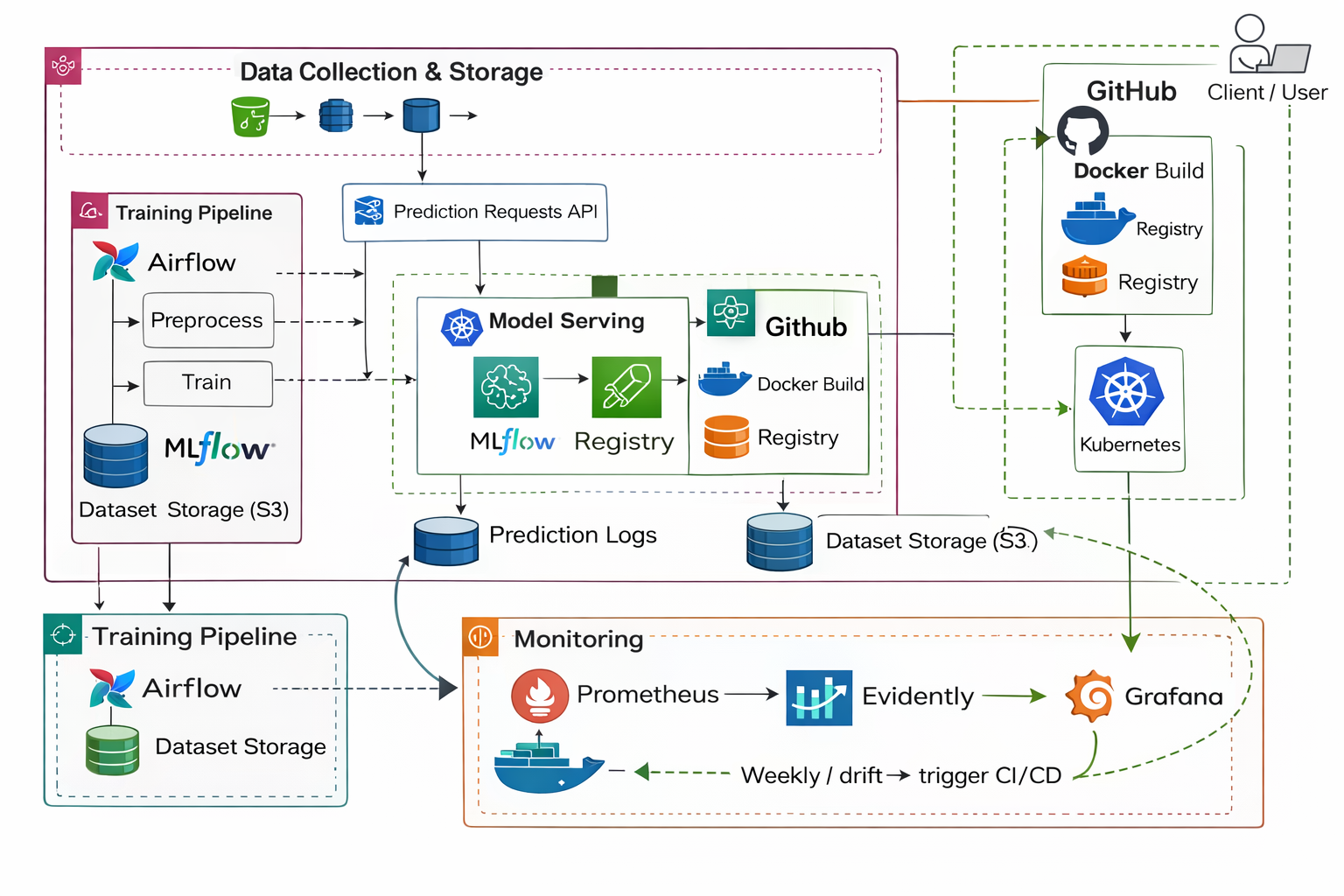
Modern machine learning in industry is not the act of training a model once and saving a file. It is the construction of a living system that keeps learning safely as reality changes. The practical lifecycle always follows the same loop: data is collected, validated, transformed, used to train a model, deployed as a service, monitored in production, and retrained when the environment changes. In mathematical form the workflow can be expressed as [ \text{Data} \rightarrow \text{Validation} \rightarrow \text{Training} \rightarrow \text{Deployment} \rightarrow \text{Monitoring} \rightarrow \text{Retraining} \rightarrow \text{Repeat}. ]
To understand this concretely we begin with a tabular medical dataset used for binary classification: predicting whether a patient has diabetes. Each record contains physiological measurements such as glucose concentration, blood pressure, insulin level, body mass index and age, and the label [ Outcome \in {0,1}. ] The critical real-world lesson appears immediately: the dataset contains impossible values such as glucose equal to zero or BMI equal to zero. These do not represent measurements but missing data. Therefore before any modeling the pipeline must transform [ 0 \rightarrow \text{missing value} \rightarrow \text{imputation}. ] This step illustrates a core MLOps principle: production failures usually originate from bad input data rather than from algorithms.
For structured tabular data, classical machine learning is preferred over deep learning. Gradient boosted trees are typically optimal because they capture nonlinear relationships without requiring large datasets. The model effectively learns a probability function [ f(X) = P(Y=1 \mid X), ] meaning the chance a patient has diabetes given measurements. The trained model and its preprocessing transformations must both be saved as artifacts because prediction later must apply identical transformations to new inputs; otherwise training and inference distributions diverge and predictions lose meaning.
Before training begins, the data must be validated with strict rules such as acceptable physiological ranges and valid label values. Validation protects the model from garbage input. After training, experiments are tracked using an experiment manager that stores parameters, metrics, and model artifacts so that different attempts can be compared. The goal is not just to train a model but to know which exact configuration produced the best performance and why. The selected model is then promoted to a production stage in a registry, meaning the system always loads the approved version rather than a random file copied manually.
The model then becomes a software service exposed through an API endpoint. A request arrives, the saved preprocessing pipeline transforms the input, and the model returns a prediction. Packaging the service inside a container ensures the same environment runs everywhere, eliminating dependency mismatches. At this moment the project stops being a notebook experiment and becomes an application.
Once deployed, a new problem appears: the system must be monitored. Two independent questions exist in production. The first question asks whether the service infrastructure is healthy. Monitoring tools measure latency, request counts and error rates to answer “Is the system alive?” The second question asks whether the model is still valid for the real world. For this we compare incoming data with the training distribution using statistical hypothesis testing. For numerical features a common test is the Kolmogorov–Smirnov test, which evaluates the null hypothesis that two samples originate from the same distribution. Each feature produces a p-value and if it falls below a threshold the feature is considered drifted. A dataset drift score can then be computed as [ \text{drift score} = \frac{\text{number of drifted features}}{\text{total features}}. ] If the score exceeds a chosen boundary such as 0.3 the system considers the model unreliable.
It is important to distinguish between new normal data, outliers, and true drift. Normal data is simply predicted and stored. Outliers such as impossible medical values are rejected before reaching the model. Drift occurs only when the overall population changes, for example when the age distribution of patients shifts. In that case the model is not replaced with a new algorithm; instead the same training pipeline is executed again using accumulated recent data. Mathematically the dataset evolves as [ D_{\text{new}} = D_{\text{old}} \cup D_{\text{production}}, ] and the model is retrained on the updated distribution.
Automation ties the entire lifecycle together. A pipeline scheduler or CI system triggers retraining when drift is detected or on a periodic schedule. A new model is trained, evaluated, registered, packaged, and deployed automatically while the running service is safely replaced. The loop therefore becomes continuous: predictions generate data, monitoring evaluates change, retraining updates knowledge, and deployment refreshes the system without human intervention.
The essence of MLOps is therefore not building a model but building a self-maintaining learning service. The model is only one component inside a feedback system that continuously observes the world and adapts to it. In simple form the discipline can be summarized as a perpetual cycle: collect data, learn from it, serve predictions, verify assumptions, and relearn when assumptions break.